Brusselator System Simulation.
Figure 1. Governing equations of the Brusselator system.
Overview
This project simulates a Brusselator reaction-diffusion system using coupled partial differential equations that describe the spatio-temporal evolution of two chemical species, \(U\) and \(V\). Where \(U(t, \mathbf{x})\) and \(V(t, \mathbf{x})\) represent chemical concentrations, \(D_U\) and \(D_V\) are diffusion coefficients, and \(A\) and \(B\) are system constants. The spatial domain is \(\Omega = [0,1]^2\), solved over the time interval \([0, T_{\max}]\) with Dirichlet boundary conditions.
Numerical Methods & Configuration
The solver employs finite difference discretization in space and Forward Euler integration
in time over a \(1024 \times 1024\) node grid
(\(\Delta x = \Delta y = 1/1024\), \(\Delta t = 0.0025\), \(T_{\max} = 1000\)).
Model parameters are \(A = 1.0\), \(B = 3.0\), \(D_U = 5 \times 10^{-5}\), and
\(D_V = 5 \times 10^{-6}\). Parallelization is achieved via OpenMP
(16 threads), and simulation results are exported as .dat files and
visualized with a Python post-processing script.
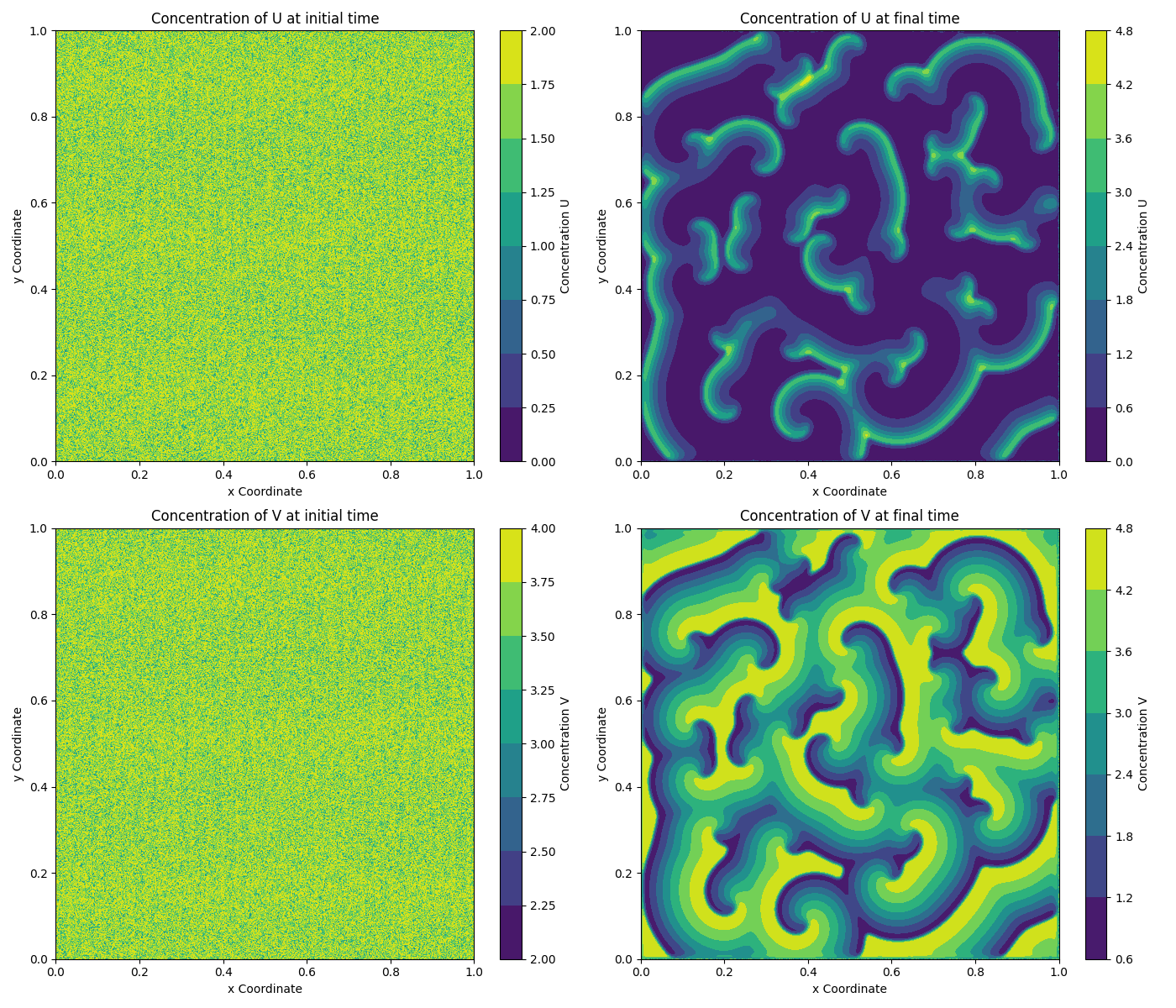
Figure 2. Simulation output — spatial concentration patterns of species U and V.